What Does a Three-Point Lead Tell Us? Survey Error and Uncertainty in Pre-Election Polling

Quick takeaways for a new survey researcher

1. Decide what you’re estimating before you collect anything

• Write one sentence: “I’m estimating [share / lead / two-party lead] among [population] at [time].”

• A poll of registered voters, one of likely voters, and a forecast of the vote are three different things. Don’t let the headline blur them.

2. Compute uncertainty for the number you actually report

• If you report a lead, compute the interval for the lead, not for one candidate’s share.

• Rule of thumb: when the race is close and two candidates take most responses, the lead’s margin is about twice the share’s margin.

• Example: 1,000 likely voters, A 48%, B 45%. Each share is about ±3.9 points, but the lead of +3 is about −4.6 to +10.6.

• For lead variance, code each respondent +1 (A), −1 (B), 0 (other) and take the standard error of that variable. With weights or clustering, use Taylor linearization or replicate weights, not the simple formula.

3. Don’t trust sample size alone

• A bigger sample shrinks random error but does nothing for bias. If one side is less likely to respond within your weighting groups, a large sample just gives you a precise wrong answer.

• A low response rate is not proof of bias, and a high one is not proof of accuracy. What matters is whether participation is related to the answer.

4. Weight carefully, and say what you did

• Start with design weights, then adjust for nonresponse and calibrate to external totals.

• Demographic weighting won’t fix partisan differences in who responds. Political weighting (party or past vote) may help on average but is not guaranteed to, so report results both ways if you can.

• Past vote is self-reported and can be misremembered. Treat it as a measured variable, not a fact.

5. Treat the questionnaire as a measurement instrument

• Ask the exact ballot question the same way every time. Don’t put issue or approval questions before it unless you’ve tested the effect.

• Use a “lean” follow-up for undecided respondents and report both the initial and the leaned numbers.

• Add a certainty question. A firm preference and a weak one are not the same data.

• If you use more than one mode, don’t assume differences are real. They can come from who responds, how they answer, or both.

6. Be honest about turnout

• Likely-voter models are assumptions. Report your headline under two or three reasonable turnout rules and show how much it moves.

• Self-reported intent to vote is usually over-reported. Don’t treat it as a reliable predictor.

7. Don’t over-trust averages

• Averaging reduces independent noise only. Errors shared across polls (same frames, same weighting, same turnout assumptions, late opinion change) stay in the average.

• In my illustration, naive 95% intervals covered the truth only about 29% of the time for an average of 100 polls when a 2-point shared error was assumed. That figure comes from assumed inputs, so treat it as a demonstration, not a measurement.

8. Report three kinds of uncertainty separately

1. Sampling precision: the interval under your design.

2. Sensitivity: how the result changes under other weighting, turnout, and undecided assumptions.

3. Prediction: how far the final result could differ from your poll, which needs a forecast model, not just the poll.

9. Minimum to disclose with every result

Sponsor, field dates, population, frame and recruitment, mode and languages, unweighted n, exact question wording and order, weighting variables and benchmarks, likely-voter rule, treatment of undecideds, and how you calculated the interval.

10. Common mistakes to avoid

• Applying a share’s margin of error to a lead.

• Calling a 2-point lead “real” because it’s inside the margin on the wrong quantity.

• Reading small changes between polls as opinion change without checking wording, mode, or weighting changes.

• Describing a poll as a prediction of the vote.

• Treating a nonprobability sample’s “margin of error” as if it came from random sampling.

A 5-minute pre-release checklist

• Can I name the estimand in one sentence?

• Did I compute the interval for the number in the headline?

• Do I know what my weighting does and doesn’t fix?

• Have I shown results under at least two turnout rules?

• Is every disclosure item above in the release?

Normal0falsefalsefalsefalseEN-USX-NONEX-NONE

Abstract

A pre-election poll can estimate each candidate’s support more precisely than the gap between them, and neither estimate automatically predicts the eventual vote. This tutorial translates total survey error into a reporting framework that distinguishes what sampling intervals, sensitivity scenarios, and predictive intervals allow readers to infer. A running district-poll example traces those distinctions from recruitment and ballot measurement through calibration and turnout modeling. Two analytic demonstrations quantify how differential participation reduces interval coverage as sample size grows and how shared errors reduce coverage as more polls are averaged. A randomized reader-study protocol tests whether a display that separates these quantities improves the corresponding judgments. The framework gives psychological researchers who lack an external outcome benchmark a way to report which conclusions depend on sampling, adjustment, and prediction.

Keywords: total survey error, election polling, nonresponse bias, survey measurement, uncertainty communication, likely-voter models

Public significance statement. A poll can estimate each candidate’s support more precisely than the gap between them. Larger samples narrow sampling intervals, but selective participation can still shift the estimates. We show how to report those sources of uncertainty separately.

1. Introduction

A poll shows Candidate A at 48% and Candidate B at 45%. The release gives a margin of sampling error of about four percentage points. Applying that margin to the three-point lead answers the wrong statistical question. The lead is a contrast between two estimates from the same respondents. Its precision depends on their covariance. Even an interval calculated for the correct contrast leaves open whether the sample represents the target population or whether that population resembles the people who will vote. These problems recur in psychological research whenever a sample statistic is used to make claims about a population or a future behavior (Groves & Lyberg, 2010).

Our aims are practical and conceptual. Practically, we give researchers a compact account of how a headline such as “Candidate A leads Candidate B, 48% to 45%” is produced and which of its components can be quantified. Conceptually, we argue that each stage of the pipeline raises a question psychology is well placed to study: how respondents construct answers (Tourangeau et al., 2000), why some people participate and others do not, and how people interpret probabilistic claims.

The total survey error framework connects choices about representation and measurement to the errors they can introduce (Groves & Lyberg, 2010). We use it to trace the three-point lead from recruitment and interviewing through weighting, turnout adjustment, and reporting.

AAPOR’s postmortems benchmark poll estimates against returns, and Keeter and Kennedy (2026) examine when political weighting can improve representation. This tutorial uses those results to locate the limits of a headline claim and makes the proposed reporting format testable. Its contribution is the link between each uncertainty display and a distinct reader inference. The derivations illustrate established statistical principles.

2. Populations and contrasts

Two decisions define a topline. First, specify the population and time: registered voters during fieldwork, an electorate modeled using expected turnout, or people who eventually cast a valid vote in the contest. Second, specify the contrast and denominator: an individual share, a lead among all included respondents, or a lead restricted to the two major candidates. A two-party margin can be reported for any of these populations. The choice of denominator is separate from the choice of population.

Certified returns directly benchmark the eventual vote margin. They cannot recover the preferences of registered voters during fieldwork. The poll-to-result discrepancy can combine coverage or nonresponse bias, measurement error, turnout misestimation, and changes after fieldwork. Identifying these components requires auxiliary evidence, such as reinterviews, records of participation, or concurrent surveys with different designs.

A national generic congressional ballot measures party preference at the national level. House seats are won district by district. Translating a national preference margin into seat probabilities requires a model of district outcomes, including the dependence of errors across districts.

3. Representation

3.1 Frames and recruitment

Probability recruitment gives frame members known nonzero selection probabilities. Common frames include address lists, telephone numbers, and voter files; each has distinct coverage properties, and a probability-recruited online panel should be described by both its recruitment mechanism and its response mode. Opt-in recruitment lacks a known selection mechanism. Pollsters compensate through quotas, sample matching, propensity modeling, or model-based poststratification. These strategies work to the extent that measured covariates capture the variables driving both selection and the outcome (the missing-at-random assumption conditional on covariates).

Fieldwork determines how much of the frame becomes observable. A voter-file text survey depends on matched phone numbers and the ability to open a web questionnaire. Address-based recruitment can use mailed invitations and offer telephone completion to people less easily reached online. Report contact attempts, incentives, languages, field dates, eligibility and completion dispositions, and exclusions for duplicate or invalid responses. Disclose exclusions by recruitment source where possible. This helps readers assess whether quality checks also removed a politically distinctive group.

3.2 Bias versus variance

Two facts about nonresponse are often conflated. A low response rate does not by itself indicate bias: bias depends on the covariance between response propensity and the outcome (Groves & Lyberg, 2010). Conversely, weighting on demographics cannot remove bias arising from differential participation by candidate preference within demographic cells. This is not merely a theoretical concern. AAPOR’s 2024 evaluation reports that for the third consecutive presidential cycle polls underestimated Republican support relative to Democratic support (AAPOR, 2025), and Pew Research Center reports evidence that Republicans have become modestly less likely than Democrats to participate in polls (Keeter & Kennedy, 2026). We treat partisan differential nonresponse as the central representation problem, while noting that the literature cannot yet say how much of the observed bias is due to it as opposed to turnout misestimation or late movement.

A meta-analysis found that response rates alone are weak guides to nonresponse bias across estimates (Groves & Peytcheva, 2008). Meng (2018) formalized how the association between recording and the outcome can dominate nominal sample size. For psychology, the implication is to study participation as an outcome with its own predictors, rather than infer representativeness from the overall completion rate.

3.3 A psychological hypothesis about participation

Trust may predict who responds even after accounting for the covariates used in weighting. One test would measure trust in a previously recruited panel, randomly vary the sponsor cue in an invitation, and record completion for every invitee. The experiment identifies the effect of the invitation and tests whether that effect varies by baseline trust. The association between trust itself and participation remains observational, and generalization beyond recruited panelists requires additional evidence.

4. Measurement

The response process comprises interpretation, retrieval, judgment, and response mapping (Tourangeau et al., 2000). Applied to ballot intention, the model implies that preferences vary in accessibility and stability. Committed voters retrieve an existing evaluation; uncommitted voters may construct one from party cues, candidate names, or considerations made salient by preceding items. Several design features therefore alter what the topline means.

Satisficing predicts that response shortcuts become more likely when cognitive demands are high relative to motivation or ability (Krosnick, 1991). A cue effect may instead reflect the accessibility of a genuine but weakly held consideration. An order effect alone cannot distinguish the mechanisms. Crossing cue placement with response burden, and measuring certainty before exposure, provides separate tests of whether cue effects track burden, commitment, or both.

Wording and context. Anchoring the question to “if the election were held today” ties the judgment to the present; naming candidates or party labels supplies cues absent from a generic ballot; placing issue or approval items first changes which considerations are accessible. These effects can be estimated with randomized split-ballot experiments and cognitive interviewing, and we recommend that large polling operations publish such experiments.

Probing. An initial “undecided” followed by a leaner question yields two measures with different meanings, expressed commitment and directional preference. Reporting both exposes how much the headline depends on the probe.

Mode. A live interview and a web questionnaire can reach different people and elicit different answers. Random assignment to mode identifies the effect of assignment on completion. Comparing answers among completers can still mix measurement differences with differential completion. A study designed to isolate measurement should minimize missing outcomes across modes and report how conclusions change under plausible assumptions about those outcomes.

Commitment. A ballot item followed by a certainty item separates preference from its strength. Reinterview designs can test whether weakly held preferences are less stable, subject to attrition and repeated-measurement effects. A single cross-section cannot distinguish within-person instability from changing sample composition across waves.

5. Adjustment and turnout modeling

5.1 Calibration weighting

In a probability design, inverse selection probabilities provide the initial weights. Analysts may adjust those weights for nonresponse and rake them to match external marginal totals. Multilevel regression and poststratification is a distinct approach. It models the survey outcome in demographic or geographic cells and averages the cell predictions using population counts. Partial pooling can stabilize sparse cells, but estimates depend on the model and on the quality of the population counts. Both approaches require credible information on the target population and adequate overlap between the sample and the groups being represented.

Wang et al. (2015) demonstrate the potential of multilevel regression and poststratification in an opt-in election sample. The empirical success of that application does not establish exchangeability within adjustment cells for other samples. Inspect sparse cells, benchmark uncertainty, and sensitivity to model specification before treating the resulting interval as a measure of population uncertainty.

In analyses of Pew Research Center’s 2020 and 2024 post-election surveys, party-affiliation weighting improved agreement with returns by roughly two to three points on the candidate margin (Keeter & Kennedy, 2026). The comparison illustrates what political calibration can accomplish with a particular benchmark. Its performance in a new pre-election survey depends on how well the benchmark describes the target population and whether the adjustment addresses the relevant selection process.

AAPOR’s 2020 postmortem found no average accuracy advantage for polls that weighted by partisanship and 2016 vote relative to polls using standard demographics alone (AAPOR, 2021). This between-poll comparison differs from Pew’s comparison of alternative weights applied to its own post-election data. Neither design isolates a general causal effect of political weighting. The benchmark can improve balance while leaving within-party differences between respondents and nonrespondents intact.

5.2 Likely-voter models

Turnout models either classify respondents by a threshold on a score or assign probabilities. With survey weight wᵢ, turnout probability qᵢ, and indicator yᵢ for support of candidate A, the probability-weighted estimate is

pA = ∑wiqiyi∑wiqi

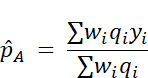
Weights govern representation; turnout probabilities govern each represented person’s contribution to the expected electorate. Validated vote records can train and evaluate turnout models, because they document participation but not candidate choice. A defensible evaluation tests out-of-sample predictions in earlier elections and checks calibration across subgroups. For live releases, reporting results under a small set of plausible turnout rules shows how sensitive the headline is to the electorate model, though scenario results remain conditional on the rules chosen.

Validated voter-file comparisons show that reports of past turnout can overstate participation (Ansolabehere & Hersh, 2012). A future intention item presents a separate measurement problem: a sincere intention can fail to translate into action, and a socially desirable answer can overstate that intention. The discrepancies have different implications for questionnaire design and turnout prediction.

Self-reported intention is an imperfect predictor of turnout. Assess its calibration against matched participation records and disclose linkage and coverage limitations. In the weighted formula above, a turnout probability estimated without candidate preference is sufficient only if residual turnout differences by preference are negligible within the predictor strata. Report sensitivity to alternatives when this assumption is consequential.

6. Uncertainty in the lead

6.1 Derivation

Under simple random sampling with a negligible sampling fraction, the variance of a candidate share is approximately the Bernoulli variance divided by sample size. The variance of the lead includes the covariance between the shares. Under multinomial sampling that covariance is negative. Coding each respondent +1 for A, −1 for B, and 0 otherwise yields the expression below.

Var(m) = pA + pB - (pA - pB)²n

For complex surveys, use Taylor linearization or the appropriate replicate weights for the contrast. The design effect compares the contrast’s variance to its variance under a specified simple random sample and can differ for the share and lead. Refit estimated adjustment or turnout models within replicates when the interval is intended to propagate their fitting uncertainty and the replication design supports it.

Unequal weighting can increase variance, but a weight-only design effect rests on restrictive assumptions and does not capture the full effects of clustering or stratification (Kish, 1992).

6.2 Worked example

Consider 1,000 likely voters with A at 48%, B at 45%, and 7% other or undecided. Assume a design effect (DEFF) of 1.6 for both shares and the contrast, equivalent here to an effective sample size of 625. A’s 95% sampling interval is 44.1% to 51.9%. The lead is +3.0 points with a standard error of 3.86 points and an interval of −4.6 to +10.6 points. The lead’s sampling margin approaches twice the share’s sampling margin when the lead is near zero and the two candidates account for nearly all responses, assuming comparable design effects. Restricting the denominator to A and B yields a separate two-party lead of about +3.2 points, with its own variance.

6.3 Differential participation and shared error

Consider an electorate that is 47% A, 46% B, and 7% other. If A supporters respond at 96% of the rate of other voters within otherwise equivalent weighting cells, the expected respondent margin is −0.90 points even though the population margin is +1.00 point. Under a normal approximation, intervals centered on the respondent estimate cover the true margin about 92%, 83%, 50% of the time at nominal sample sizes of 1,000, 4,000, and 16,000, respectively (Appendix A).

Sampling standard error decreases in proportion to 1/√n under a fixed design effect. The selection bias in this example stays at −1.90 points. At large sample sizes, repeated estimates can therefore cluster tightly around the wrong value. Calibration to the correct cell sizes leaves the discrepancy intact when it arises within the cells.

Figure 1

Coverage of a Nominal 95% Interval Under Differential Participation

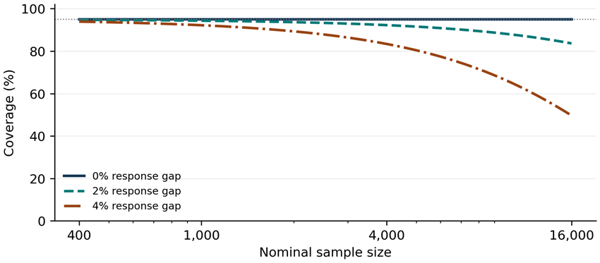
Note. Curves use the fixed-variance normal approximation in Appendix A. Gaps are relative reductions in response probability for Candidate A supporters. The dotted line marks nominal coverage.

Now suppose polls have independent sampling errors and share a mean-zero Gaussian error that varies across hypothetical races, with a standard deviation of two points. If each poll has a sampling standard error of about 3.9 points, nominal 95% intervals that ignore the shared component have approximate coverage of 92%, 80%, 56%, 29% when averaging 1, 5, 20, and 100 polls. These percentages average over hypothetical races. Within one race, the shared error is the same for every poll and remains in the average.

Figure 2

Coverage When Poll Averages Ignore Shared Error

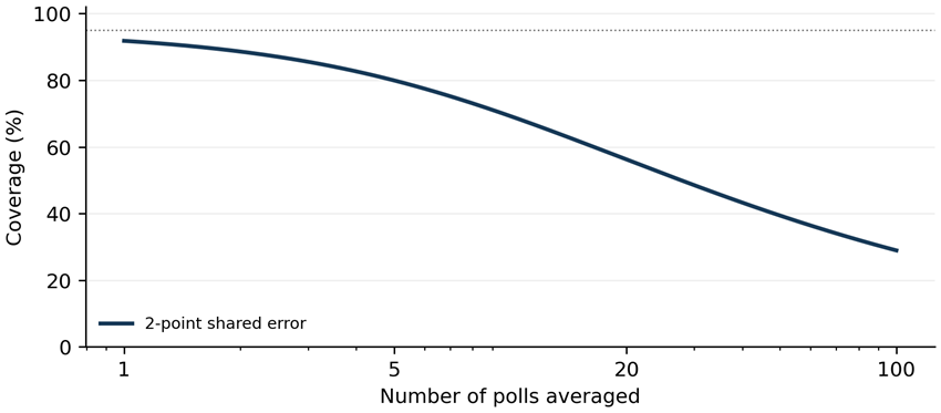
Note. Coverage averages over hypothetical races. Poll-specific sampling errors are independent. A common error with a standard deviation of two percentage points is shared by all polls in each race.

The response gap and common-error scale are illustrative inputs. Estimating either quantity for a particular election would require additional evidence.

7. What the empirical record shows

AAPOR (2025) evaluated 611 publicly released polls fielded in the final two weeks of the 2024 campaign across presidential, Senate, gubernatorial, and House contests. The mean absolute error on the two-party margin was 3.3 percentage points, compared with 5.3 in 2020 and 5.2 in 2016. The mean signed error was +2.7 points on the Democratic margin in 2024. The absolute error summarizes magnitude and the signed error summarizes direction. Neither provides the coverage probability of a sampling interval for an individual poll.

Shirani-Mehr et al. (2018) examined 4,221 state-level polls across 608 contests and found a substantial race-level component of error. This historical finding concerns disagreement with election returns. The near-twofold ratio in Section 6.2 comes from the covariance of candidate shares and can arise even under unbiased simple random sampling. Historical discrepancies can inform forecast calibration when the comparison elections are relevant and dependence is modeled.

Methodologically, hundreds of polls in one cycle do not provide hundreds of independent tests of election-level accuracy, because polls cluster within races and share errors. Evaluations should treat races and cycles as the unit of analysis, report signed error, absolute error, and interval coverage separately, and validate the specific estimand the method claims to estimate.

A pre-election archive was captured from Polling Forecast on November 2, 2026, at approximately 9:01 p.m. Eastern. Its 4,015 source records yield 309 candidate rows across House, Senate, and gubernatorial races with fieldwork ending October 20 through November 2. The companion archive preserves the source bytes, checksum, and initial eligibility rule. These are source rows, which may include multiple questions or populations from the same fieldwork. The archive is bounded by the source and capture time.

Before accessing certified returns, verify that each row concerns the general election, resolve race and candidate identities, select the main likely-voter ballot when multiple populations or questions share fieldwork, and log duplicates and exclusions. Recover the published candidate figures and denominators from original releases. Compute two-party margins from the two named major-party candidates and compare them with certified shares on the same denominator. Report the mean signed and absolute errors with equal race weighting and provide poll-weighted estimates as a sensitivity analysis. Report interval availability and compare each interval only with its corresponding result quantity. Race resampling describes between-race variation within this archive. A single cycle cannot estimate between-cycle uncertainty. Poll-to-result interval agreement includes turnout and preference change and therefore cannot validate coverage for field-period opinion.

8. A reporting standard and a research agenda

8.1 Three-layer uncertainty reporting

Non-probability polls lack a design-based margin of error; resampling respondents quantifies variability conditional on the observed sample and procedure but does not measure how far volunteers differ from nonvolunteers.

Worked release. In the illustrative district poll, A leads by 3.0 points among modeled likely voters. The approximate 95% sampling interval for the lead is −4.6 to +10.6 points. To illustrate turnout sensitivity, suppose two equally represented groups have within-group margins of +13 and −7 points. Equal turnout yields +3.0 points. Under alternative turnout models in which the first group supplies 40% or 60% of the modeled electorate, the margin becomes +1.0 or +5.0 points. These are scenario estimates. If a separate forecast assumes the poll is unbiased for the eventual margin and adds an independent, mean-zero normal forecast discrepancy with a placeholder standard deviation of 3.0 points, chosen solely to illustrate the calculation, its illustrative 95% predictive interval is −6.6 to +12.6 points. An operational forecast would need to justify and validate that discrepancy model on held-out elections.

8.2 Minimum disclosure

Release the sponsor, field dates, geography, target population, frame and recruitment, mode and languages, unweighted n overall and for key subgroups, a defined participation metric, exact question wording, order and probe, weighting variables and benchmarks, trimming, the likely-voter rule, treatment of missing and undecided responses, and the variance method. Where privacy permits, release code and replicate weights. Comparisons across waves should estimate uncertainty of the change directly, account for panel overlap, and document changes in wording, mode, screens, or weights before attributing differences to opinion change.

Uncertainty formats can affect how readers interpret evidence (van der Bles et al., 2019). A plausible prediction is that labeling an interval by its target helps readers distinguish a range for current support from a range for future votes. Whether the added information improves understanding or increases cognitive load is an empirical question.

Van der Bles et al. (2019) distinguish forms of uncertainty and examine how they are communicated. Westwood et al. (2020) test how election win probabilities change beliefs and behavior. Here the proposed test varies whether the same poll and forecast are displayed as distinct inferential targets. It scores three separable errors: treating the current lead as settled, treating a turnout scenario as a probability statement, and treating a range of future vote margins as a win probability. The format succeeds if it improves these judgments, even if perceived certainty and trust remain unchanged.

8.3 Research agenda for psychologists

Study 1. Interpretation of uncertainty. Randomly assign readers to a conventional share interval, a lead interval, or a display with a lead interval, turnout scenarios, and a forecast interval. Predict that the lead interval improves recognition that the current population lead could be zero, and that the layered display improves recognition of turnout dependence and the distinction between a predictive interval and a probability of winning. Score comprehension by claim type. Record confidence after each answer and test numeracy as a prespecified moderator.

Analysis plan. Randomize 1,500 U.S. adults equally across the three displays, using fictional candidates and counterbalanced party labels. Use one primary contrast at two-sided α = .05: layered versus lead-only on a four-item score covering turnout dependence and forecast interpretation. Code skipped items as incorrect in the primary analysis and report a completer sensitivity analysis. With 500 per arm, the normal approximation gives 80% power at about d = .18. This is a sensitivity threshold, not an expected effect. A one-quarter-item increase in the group mean is a provisional practical benchmark, equivalent to one additional correct answer per four readers on average. Pilot item difficulty and score variance before fixing the final sample size. Treat lead-only versus share-only on current-margin comprehension and all moderation tests as secondary.

Study 2. Preference construction. Cross randomized issue-item placement with a burden manipulation. The high-burden arm completes an unrelated digit-memory task while answering the ballot item. The control arm completes the same task after answering. Measure prior preference and certainty in an earlier wave. Predict that the cue shifts immediate choice more under burden and, separately, among people with lower baseline certainty. Use a common ballot item at follow-up to estimate switching as a secondary outcome. Prespecify a cue-by-burden difference in differences on the binary endorsement scale as primary. With 400 analyzable respondents per cell and probabilities near .50, a two-sided .05 test has approximately 80% power for a 14-point interaction. Smaller interactions require more respondents. Report missing responses and follow-up attrition by arm.

Study 3. Trust and participation. Measure trust in two institutions in a prior panel wave. Randomize which institution is named as the sponsor in otherwise identical invitations, using truthful sponsorship descriptions. Predict that completion increases when the assigned sponsor is the institution that the invitee rated more trustworthy. Estimate the assignment-by-signed-trust-difference interaction and report predicted completion differences. Completion is defined for every randomized invitee. For planning, among invitees with a clear trust preference, 400 per assigned condition would detect about a 9-point completion difference with 80% power at two-sided α = .05 if baseline completion is near .30. This calculation concerns the preferred-versus-other sponsor contrast. Plan interaction power separately using pilot estimates of trust dispersion and the fraction with a clear preference.

9. What transfers to psychological surveys

Consider an opt-in study estimating the prevalence of clinically significant distress among U.S. adults. Define the target population, measurement window, and screening threshold before recruitment. Report the unweighted opt-in estimate and show how it changes after calibration to demographic targets. If participation still depends on distress within those groups, increasing the sample size can tighten an interval around a biased estimate (Meng, 2018). Show sensitivity to plausible within-group selection differences and distinguish that exercise from the model-based interval. A screen-positive proportion also answers a different question from the prevalence of diagnoses established in structured interviews.

A psychological study may have no equivalent of certified returns. Use the best available checks at each stage: a reinterview to assess measurement stability, a probability reference survey to assess composition, or linked clinical interviews to assess classification in a validation subset. Each check addresses a different uncertainty. In the absence of a suitable future outcome, report sampling or model precision and sensitivity to adjustment assumptions. Add a predictive interval only when a defined future outcome and a defensible predictive model exist.

10. Limitations

The evidence is primarily from U.S. elections. Institutional reports from AAPOR and Pew provide timely evidence, with different designs and standards of review from peer-reviewed articles. The illustrations assume a fixed design effect, a specified within-cell response gap, and Gaussian shared errors. They establish consequences of those assumptions. They do not estimate the frequency or magnitude of these mechanisms in any particular election. None of the proposed psychological hypotheses or display effects has been tested here.

11. Conclusion

A ballot item measures a stated preference, a sampling and adjustment procedure estimates its distribution, and a turnout model projects it onto a possible electorate. The strongest reporting starts by naming that estimand and computing uncertainty for the exact contrast being communicated. When results depend on uncertain modeling choices, show the resulting changes in the estimate. When the claim concerns a future vote, report the assumptions and validation appropriate to a forecast.

Appendix A   Reproducing the Analytic Illustrations

Differential participation. Set g = 1 − 0.47d, a = 0.47(1 − d)/g, b = 0.46/g, and m = a − b. With nominal sample size n and fixed design effect 1.6, define s = √[(a + b − m²)/(n/1.6)] and z = (0.01 − m)/s. Approximate coverage is Φ(z + 1.96) − Φ(z − 1.96), where Φ denotes the standard normal cumulative distribution function. This is an analytic approximation with the respondent-pool variance held fixed. For d = .04, coverage at n = 400, 1,000, 4,000, and 16,000 is 93.9%, 92.2%, 83.4%, 49.7%. Setting d = 0 yields approximately 95% throughout.

Poll averaging. For k polls, set s = √[(.93 − .01²)/(625k)]. Assume each race has a shared N(0, .02²) deviation independent of poll-specific errors. The average has standard deviation √(s² + .02²). The coverage of an interval with half-width 1.96s is 2Φ[1.96s/√(s² + .02²)] − 1. At k = 1, 5, 20, and 100, coverage is 91.8%, 80.0%, 56.2%, 28.9%.

References

American Association for Public Opinion Research. (2021). 2020 pre-election polling: An evaluation of the 2020 general election polls. https://aapor.org/wp-content/uploads/2022/11/AAPOR-Task-Force-on-2020-Pre-Election-Polling_Report-FNL.pdf

American Association for Public Opinion Research. (2025). Task Force on 2024 pre-election polling: An evaluation of the 2024 general election polls. https://aapor.org/wp-content/uploads/2025/10/AAPOR-Task-Force-on-2024-Pre-Election-Polling_Report.pdf

Ansolabehere, S., & Hersh, E. (2012). Validation: What big data reveal about survey misreporting and the real electorate. Political Analysis, 20(4), 437–459. https://doi.org/10.1093/pan/mps023

Groves, R. M., & Lyberg, L. (2010). Total survey error: Past, present, and future. Public Opinion Quarterly, 74(5), 849–879. https://doi.org/10.1093/poq/nfq065

Groves, R. M., & Peytcheva, E. (2008). The impact of nonresponse rates on nonresponse bias: A meta-analysis. Public Opinion Quarterly, 72(2), 167–189. https://doi.org/10.1093/poq/nfn011

Keeter, S., & Kennedy, C. (2026, September 16). Weighting polls on party affiliation and past vote. Pew Research Center. https://www.pewresearch.org/methods/2026/09/16/weighting-polls-on-party-affiliation-and-past-vote/

Kish, L. (1992). Weighting for unequal Pᵢ. Journal of Official Statistics, 8(2), 183–200.

Krosnick, J. A. (1991). Response strategies for coping with the cognitive demands of attitude measures in surveys. Applied Cognitive Psychology, 5(3), 213–236. https://doi.org/10.1002/acp.2350050305

Meng, X.-L. (2018). Statistical paradises and paradoxes in big data (I): Law of large populations, big data paradox, and the 2016 US presidential election. The Annals of Applied Statistics, 12(2), 685–726. https://doi.org/10.1214/18-AOAS1161SF

Shirani-Mehr, H., Rothschild, D., Goel, S., & Gelman, A. (2018). Disentangling bias and variance in election polls. Journal of the American Statistical Association, 113(522), 607–614. https://doi.org/10.1080/01621459.2018.1448823

Tourangeau, R., Rips, L. J., & Rasinski, K. (2000). The psychology of survey response. Cambridge University Press. https://doi.org/10.1017/CBO9780511819322

van der Bles, A. M., van der Linden, S., Freeman, A. L. J., Mitchell, J., Galvao, A. B., Zaval, L., & Spiegelhalter, D. J. (2019). Communicating uncertainty about facts, numbers and science. Royal Society Open Science, 6(5), Article 181870. https://doi.org/10.1098/rsos.181870

Wang, W., Rothschild, D., Goel, S., & Gelman, A. (2015). Forecasting elections with non-representative polls. International Journal of Forecasting, 31(3), 980–991. https://doi.org/10.1016/j.ijforecast.2014.06.001

Westwood, S. J., Messing, S., & Lelkes, Y. (2020). Projecting confidence: How the probabilistic horse race confuses and demobilizes the public. The Journal of Politics, 82(4), 1530–1545. https://doi.org/10.1086/708682