Candidate Appeal and Reasons to Oppose an Electoral Opponent

Quick Takeaways

The question: When voters say they voted “against” a candidate, is it because they dislike the opponent, or because they weren’t excited about their own pick? This paper asks something narrower: if voters like their candidate more, do they care less about stopping an opponent who looks more threatening?

Why it matters: About three in ten U.S. voters in 2020 described their vote as more “against” than “for.” That rate was 15% among strong partisans but over 50% among independents and leaners. These numbers come from one survey taken after the election, so we don’t yet know the cause.

The plan: This is a proposed experiment that has not been run, so there are no results yet. Participants would read short descriptions of fictional local elections. The researchers would randomly vary two things:

• how appealing the voter’s preferred candidate is (routine involvement versus concrete follow-through on constituents’ concerns), and

• how threatening the opponent is (respecting, delaying, or blocking an independent oversight check).

Participants would then rate how much each reason would matter to their vote: electing their candidate and stopping the opponent.

What would count as an answer:

• A more appealing candidate weakens the effect of the threat (buffering).

• It strengthens it (amplification).

• It makes no practical difference, because the two simply add up.

Built-in safeguards: The design guards against a false buffering result caused by the rating scale itself and tests that safeguard with simulated data. It also separates the candidate’s appeal from the issue the voter cares about.

Limits: It measures reported reasons in a simulated election, and it doesn’t show what drives real votes. Results would apply only to these kinds of threats and appeals.

Abstract

Voters can support the same candidate while placing different weight on electing that candidate and defeating the opponent. Observational research links opposition-centered voting to weaker positive candidate evaluations and weaker partisan identification. It remains unclear whether a more appealing candidate reduces the weight voters give to stopping the opponent as a threat increases. We propose a 2 × 3 survey experiment that crosses aligned-candidate appeal with three levels of opponent threat across 36 fictional election profiles. The appeal and threat cues concern different behaviors and are independent of the policy used to establish candidate alignment. Separate ratings allow respondents to endorse both reasons strongly or neither. The primary outcome is the independently rated importance of stopping the opponent. A prespecified interaction contrast distinguishes attenuation, amplification, and practically negligible effects on that scale. An intermediate threat level, response distribution diagnostics, and a bounded-scale sensitivity model address the possibility that apparent attenuation reflects response compression. Confidence intervals quantify respondent assignment uncertainty within the fixed stimulus bank. Generalization to other threat and appeal cues requires new evidence. The proposed study tests reported reasons in a simulated election. It has yet to be fielded.

Keywords: negative voting, candidate evaluation, partisan identity, vote rationale, survey experiment

Introduction

A vote for a candidate can express endorsement, opposition to the alternative, or both. Consider two voters who support the same candidate. One wants that candidate in office and is also deeply concerned about what the opponent would do. The other sees little reason to endorse either candidate and votes mainly to prevent a particular outcome. Both could describe the vote as more against than for. That description alone cannot tell us how important opposition was in absolute terms or whether stronger support would have changed its importance.

Garzia and Ferreira da Silva (2022a) asked respondents, “Would you say your vote is more a vote for Trump [Biden] or more a vote against Biden [Trump]?” In their online panel of 1,064 respondents, fielded November 9–29, 2020, 30.2% of those who reported voting characterized their ballots as votes against. Negative framing was reported by 15% of strong partisans, 37% of weak partisans, and more than half of leaners and independents. Candidate evaluations were more closely associated with framing than party evaluations in their joint model. The gap in evaluations of the supported candidate was also larger than the gap in evaluations of the opponent. Those results come from a single post-election survey conducted after the projected winner was known. Voters could have reconstructed their reasons in light of the outcome, and the forced comparison could not distinguish mixed motives from indifference. The survey also found a substantial candidate asymmetry, with 39% of Biden supporters and 18% of Trump supporters reporting negative votes. Zheng’s (2025) preprint offers further evidence of asymmetry using a separate operationalization. These patterns are reasons to avoid inferring a symmetric causal effect from the 2020 data.

Garzia and Ferreira da Silva’s composite framework integrates evaluations, partisan identity, and retrospective judgments (2022b), and their subsequent work examines negative voting in Canada, France, Germany, the Netherlands, and the United States (2024). Across five studies, Siev et al. (2024) likewise found that independents were more likely than partisans to hold or express electoral preferences grounded in opposition. That work includes tests of preferences for messages framed around support or opposition. The present study asks a different causal question. When the same evidence about the opponent is supplied to voters, does favorable information about the alternative change the effect of that evidence on the importance they assign to stopping the opponent?

Why candidate appeal could change sensitivity to threat

Positive and negative evaluations can coexist and vary partly independently (Cacioppo & Berntson, 1994). Applied to a candidate pair, this suggests that enthusiasm for electing one candidate and opposition to electing the other need not trade off. An additive account predicts that the threat cue increases the reported importance of stopping the opponent by roughly the same amount across appeal conditions. Appeal may increase the importance of electing the aligned candidate and could shift which reason dominates, even if the opposition rating barely changes. Under this account, a shift toward support-centered framing need not imply reduced sensitivity to threat.

Reason-based choice proposes that people construct reasons to resolve a difficult choice and justify it to themselves or others (Shafir et al., 1993). Ambivalence research likewise suggests that approaching a decision can make mixed evaluations uncomfortable and motivate people to resolve that conflict (van Harreveld et al., 2009). Applied here, a credible positive case for the aligned candidate may settle the prospective ballot early, making additional opponent information less useful as a reason for that ballot. When the affirmative case is weak, the same information can resolve an otherwise unsettled choice. Reason-based choice also permits additive reasons, and the ambivalence model describes mixed evaluation of one object. Applying it to a choice between two candidates requires the additional assumption that uncertainty about the ballot creates a similar motive for resolution. That extension motivates a specific prediction: attenuation should appear on an independent opposition rating, even when voters can endorse both reasons. The experiment tests that prediction. It does not observe when a choice was settled or whether participants allocated less attention to the threat.

A competing amplification account starts from what is at stake. If voters regard an appealing candidate’s victory as especially desirable, an opponent who could prevent it may make opposition feel more consequential. Threat and appeal would then reinforce each other. A separate possibility is response compression. A bounded scale can flatten a treatment response near its endpoints even when the underlying effects are additive. This possibility matters for the interpretation of an interaction and is distinct from a practically negligible interaction on the observed scale.

The partisan gradient motivates a secondary question. Strong identifiers may have an affirmative reason to support a candidate before hearing anything about either profile. Independent leaners may share a policy preference without that stable source of affirmation. These groups may differ in opposition-centered framing even if the experimental appeal manipulation has identical effects for both. Accordingly, partisan strength is a measured moderator, and group differences do not identify the causal effect of partisan identity. Baseline party affect and felt ambivalence are measured separately. Coldness toward the less preferred party is not equivalent to weak warmth toward the preferred party, and feeling torn is distinct from having little feeling about either party.

Hypotheses and decision rules

The primary outcome is the importance assigned to stopping the opponent on an independent 0–100 rating. The comparative “for versus against” label is secondary. The intervention concerns stated threats to institutional checks in a simulated local election. The study does not estimate the prevalence of negative voting, responses to policy loss, or affective aversion. Let Δ equal the high-minus-low threat effect under enhanced appeal minus the high-minus-low threat effect under ordinary appeal, averaging equally over the profile bank and measurement orders.

H1. Buffering predicts Δ < 0, alongside a positive threat effect under ordinary appeal. H2. Amplification predicts Δ > 0, alongside a positive threat effect under enhanced appeal. A two-sided 95% confidence interval entirely below or above zero establishes direction. The ±5-point equivalence margin addresses practical size, so a precisely estimated small directional effect can also be equivalent. The relevant positive simple effect must also have a two-sided 95% interval above zero to interpret the pattern as attenuation or amplification of a positive threat response. If the threat effects have opposite signs, the pattern is described as a threat-effect reversal. This is distinct from plotted lines crossing when appeal changes which line is higher.

H3. Practical additivity on the observed scale predicts a 90% confidence interval for Δ fully within ±5 rating points, using two one-sided tests at α = .05 (Lakens, 2017). Directional and equivalence decisions can coexist when an effect is precisely estimated and small. An interval crossing zero and either equivalence bound is inconclusive. Five points is one third of a prespecified 15-point high-minus-low threat benchmark. Fifteen points is a design target for a substantively useful threat manipulation, not an empirical estimate. If the pilot does not rule out effects of 10 points or less, the confirmatory study will not proceed under this design. The compression account is a rival interpretation. The reporting hierarchy and its limitations are specified below and evaluated using synthetic data.

Table 1. Outcomes and decision rules

Figure 1

Predicted opposition ratings across opponent threat levels

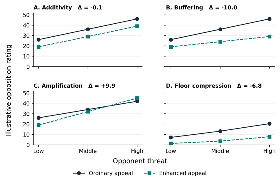
Note. Illustrative values only. Panels A–C share low-threat baselines. Panel C has an interaction of about +10 points. Panel D uses lower baselines to show floor compression: the same latent threat increments produce different observed increments after rounding and clipping. The panel uses the logistic generator in Supplement S1.

Method

Sample and assignment

The proposed source is a U.S. opt-in online panel with prescreening for voting eligibility, age 18 or older, and English reading proficiency. Recruitment will use quotas for age, gender, and party identification, including unaffiliated respondents. The sampling design supports comparisons within the recruited population. National prevalence estimates are outside its scope. Before assignment, respondents indicate their policy preference and its strength across the policy domains. Eligibility requires a directional preference on at least one domain. The study records party identification on the standard seven-category branching measure, party feeling thermometers, and a direct rating of how torn respondents feel about the parties. Pure independents without a party preference are included in the primary analysis. Their party affect is summarized separately when a preferred party cannot be defined.

The fixed bank crosses four policy domains (transit, libraries, flood mitigation, and recreation), three institutional threat types, and three appeal cue pairs, yielding 36 sets. Each set has two mirrored policy versions so alignment follows pretreatment preference. Candidate names and display order are counterbalanced. When multiple domains are compatible, the instrument selects uniformly among the respondent’s compatible domains that have open quotas, then among open compatible sets within the selected domain. If all compatible quotas are closed, the respondent is not randomized. Recruitment can target underfilled domain-by-preference strata using screening responses only. Within each set and mirrored version, independent randomized blocks of 12 cover every treatment-by-order combination. Incomplete final blocks are retained. Quotas govern randomized starts, and completion imbalances are reported by cell. A feasibility check before the main study will determine whether the planned mirrored-version quotas can be filled. Any revision to the bank or quotas will occur before confirmatory recruitment.

Experimental materials and validation

Alignment comes from a shared policy position that neither treatment modifies. Threat types are interference with ethics review, obstruction of a public audit, and suppression of a legally required public report. Each has a low, intermediate, and high level corresponding to respect for the safeguard, a temporary discretionary delay, and a unilateral block. Appeal pairs vary substantive evidence of responsiveness in three settings: a public meeting, a constituent help desk, and an advisory forum. The enhanced versions show concrete follow-through with documented outcomes or next steps, while ordinary versions show competent routine participation. Both candidates’ descriptions will be matched in length and specificity where possible. The Appendix specifies all six cue families and how they are crossed. Multiple exemplars reduce dependence on a single vignette, but three deliberately chosen families cannot support inference to a population of threat or appeal wordings (Judd et al., 2012).

The independent pilot targets 2,160 analyzable responses, 60 per set or 240 per threat dose within each threat family. For a standardized adjacent-dose contrast within family, the nominal 90% interval half-width is about .15 SD under equal allocation and unit variance. For an appeal contrast within family, the corresponding half-width is about .12 SD with 360 per appeal level. Adjacent threat levels will be checked using the pooled gate below, and family estimates will screen for reversals rather than certify equivalence. A separate 0–100 liking thermometer checks whether the cue improves overall liking as well as perceived responsiveness. Three items each measure perceived appeal and threat. The two-factor model must improve comparative fit index by .01 over a one-factor model, and the upper 95% bound on the absolute factor correlation must be below .85. The lower 90% bound must exceed .30 pooled within-cell SD for the appeal cue on the appeal composite, .20 SD on liking, and .15 SD for each adjacent threat contrast on perceived threat. Pooled 90% intervals for cross-cue shifts in appeal or threat and for cue effects on viability and perceived policy alignment must fit inside ±.20 SD. Family-level point estimates will be checked for reversals or spillovers exceeding .30 SD in absolute value. As an outcome-scale feasibility check, the marginal high-minus-low opposition effect averaged across appeal levels must have a one-sided 90% lower confidence bound above 10 points. At a planning SE of 1.32 points, this requires an estimate above 11.69 points and passes about 99% of the time when the true effect is 15, versus 10% when it is exactly 10. Fifteen points remains the design benchmark and five points remains the fixed equivalence margin. This gate does not inspect any outcome interaction. Pilot participants are excluded from the main study.

A provisional six-to-eight-week window after ethics clearance allows two weeks for initial fielding, one week for diagnosis, one to two weeks for revisions and any necessary review, and two to three weeks for one independent repilot. These are planning allowances. If the repilot fails the same gates or compatible quotas prove infeasible, the main study pauses for a revised Stage 1 plan.

Outcomes and measurement order

Respondents will be randomly assigned to complete the simulated ballot either before or after the rationale block. Ballot options include both candidates and abstention. In both orders the rationale block starts with an open prompt: “If you were to vote for [aligned candidate], what considerations would matter to you?” All respondents then rate two considerations independently on 0–100 scales anchored by “would not matter at all” and “would matter a great deal”: electing the aligned candidate and preventing the opponent from taking office. The item order is randomized. The opposition rating is primary. The support rating is a key secondary outcome. Both can be high or low. A subsequent comparative item offers five categories: mostly electing the aligned candidate, mostly stopping the opponent, both about equally, neither, and another reason or unsure. “Neither” is reported separately. Two coders blind to assignment classify open-ended responses for mention of support and opposition independently, with an adjudication rule fixed before coding and agreement reported before adjudication.

Reason reports have two distinct limitations. Respondents may have incomplete access to the processes underlying their decisions (Nisbett & Wilson, 1977), and eliciting reasons can itself alter choices (Wilson & Schooler, 1991). Mummolo and Peterson (2019) found limited experimenter demand effects in the survey experiments they examined. That result does not establish that naming motives leaves this instrument unaffected. The open prompt precedes named reasons, the ballot order is randomized, and a final purpose probe records perceived expectations. Effects remain causal effects of the vignette on reported reasons. Vote choice is analyzed in all assigned respondents with an observed ballot, separately from the rationale. No primary analysis conditions on which candidate the respondent chooses.

Analysis, precision and exclusions

The primary analysis targets the equally weighted average over the 36 fixed sets, their two mirrored versions, and both measurement orders. Each component contrast comes from the four relevant extreme-dose means. Index the 144 profile-by-mirror-by-order strata by h, and order the four extreme cells as ordinary low, ordinary high, enhanced low, enhanced high. With c = (+1, −1, −1, +1) and wₕ = 1/144, the estimator and variance approximation are:

Δ̂ = Σₕ wₕ Σⱼ cⱼ Ȳₕⱼ

V̂(Δ̂) = Σₕ wₕ² Σⱼ cⱼ² sₕⱼ² / nₕⱼ

Here nₕⱼ and sₕⱼ² are the observed cell count and sample variance. The variance is a Neyman-style approximation using the analysis strata and omitting the unidentifiable finite-population contrast variance under complete random assignment within strata. With incomplete blocks and outcome loss, it is a working approximation rather than an exact design guarantee. A normal interval is used for the aggregate contrast. If an extreme-dose cell has fewer than two observations, pool both measurement orders for that mirror across all six arms and give the pooled group weight 1/72. If an extreme-dose cell remains sparse after order pooling, pool both mirrors and orders for that profile across all six arms and give it weight 1/36. If an extreme cell is still sparse, report the affected profile and treat confirmatory inference as unavailable. Do not silently drop profiles or borrow from other profiles. Report which strata were pooled and the realized composition by arm. Pooling preserves profile weights but substitutes realized order or mirror mixtures for equal weights within affected groups. If pooling occurs, report the result with that qualification and show a complete-strata sensitivity estimate labeled as a different target. Report all six marginal means, both simple effects, adjacent contrasts, and contrasts by appeal family and threat family. Re-estimate Δ leaving out each family in turn to show dependence on any one implementation. These are robustness descriptions. The uncertainty interval pertains to respondent assignment within the bank, and does not estimate how effects would vary over a larger stimulus population.

The nominal main-study allocation is 9,072 randomized starts (252 per set, 126 per mirrored version), with up to 10% loss anticipated. The sensitivity table uses a conservative rounded planning count of 8,100 observed outcomes. With equal allocation across six cells, the interaction standard error is √(24σ²/N), and either simple-effect standard error is √(12σ²/N), where σ is the within-cell rating SD. The full directional decision requires both a 95% interaction interval excluding zero in the predicted direction and a 95% simple-effect interval above zero. The table reports joint power using correlated normal estimates, because the simple effect and interaction share two cell means. The scenarios use a five-point interaction and a positive reference simple effect of either 15 points (design target) or 5 points (stress test). At a true zero interaction, equivalence power is the chance that the 90% interval falls entirely within ±5 points. These are conditional-bank calculations. There is no assumed between-set interaction SD and no attempt to estimate it from a shallow pilot. Only pooled within-cell variability, completion, and quota feasibility will inform whether the nominal cap is retained. If the blinded nuisance estimates imply less than 80% power for either the design-target joint decision or equivalence, the cap or design must be revised in Stage 1 before main-study recruitment. The final randomized-start cap will be registered before fielding, with no outcome-based stopping.

Table 2. Power sensitivity within the fixed stimulus bank

Note. Joint columns require a five-point interaction and a positive reference simple effect, whose true value is 15 or 5 points. Equivalence assumes a true zero interaction.

Eligibility and a single instructional check are assessed before randomization. Panel-verified duplicate or fraudulent entries identified using prespecified, assignment-blind rules are removed. Respondents are retained regardless of post-treatment comprehension, speed, or inferred study purpose. Report exclusions, outcome missingness, and completion by arm. The primary estimate uses observed ratings. Sensitivities use arm-specific multiple imputation from pretreatment variables, profile and survey order under missing at random, and bounded worst-case assignments for missing ratings to show how much attrition could move the contrast.

The secondary family comprises the support-rating interaction, the open-ended opposition-mention interaction, and the effect of randomized measurement order on aligned-candidate choice. Apply Holm adjustment across these three tests. Report the full comparative-item distribution and the full ballot distribution by cell with descriptive intervals. Prespecified exploratory moderation examines identity strength, prior affect toward the less preferred party where defined, and felt ambivalence. Fit each separately with all lower-order terms. Report effect estimates and intervals, with Holm adjustment across the three interaction tests. The study is powered for the average contrast. Subgroup uncertainty will be reported even when estimates appear to differ.

Compression and simulation checks

Report directional and equivalence tests separately. For either directional call, fit the common-threshold additive ordinal model to the pooled counts in the seven prespecified rating bands (0, 1–24, 25–49, 50, 51–75, 76–99, 100) and compare it with the saturated treatment-cell band model. Also test additivity on the logit of the six marginal mean ratings divided by 100. The latter test uses a two-degree-of-freedom delta-method Wald test for equality of the two adjacent threat increments across appeal conditions, using the weighted cell means and their estimated variances. Neither model uniquely identifies the response scale or a latent mechanism.

For a single summary label, practical equivalence has priority. Otherwise, a directional result is compression-compatible if either benchmark yields p ≥ .05. This label records compatibility with at least one additive benchmark and does not establish compression. If neither is compatible and either model is unavailable, report that the diagnostic is incomplete. Otherwise retain the directional label. Append an endpoint warning if at least one pooled cell has 20% or more of ratings at 0 or 100 combined. This descriptive cutoff means at least one in five ratings cannot move farther toward its chosen endpoint and is a heuristic for conspicuous saturation. Report the actual percentages. Endpoint frequency never determines whether to run a model. Sparse ordinal bands and pooling across profiles can limit the likelihood-ratio approximation.

Supplement S1 reports the synthetic validation, including a beta-distributed compression scenario with no clipping. Its executable script fixes the generator parameters, seed and reporting rules for review. The main-study registration will archive those exact versions alongside the finalized analysis workflow before recruitment.

What each result would change

If greater appeal weakens the threat effect on an independently rated opposition motive, the result would extend the literature beyond the finding that candidate liking predicts whether a voter chooses a “for” or “against” label. Convergence with spontaneous mentions and a pattern poorly captured by additive scale compression would strengthen that interpretation. An equivalent interaction alongside a clear increase in support would favor an account in which voters gain an affirmative reason while retaining their reasons for opposition. Amplification would suggest that a valued alternative can raise the perceived stakes of stopping its opponent.

Viability matters because strategic voting depends on preferences and beliefs about which candidates can win (Blais & Nadeau, 1996). Holding stated viability constant and checking inferred viability reduces one competing explanation. It does not remove all strategic reasoning. Fictional candidates also reduce the influence of retrospective performance and longstanding candidate identities. These controls limit generalization to real campaigns, where party cues, strategic incentives, incumbent performance and post-election rationalization can all shape reported reasons. Even with a clean pilot, the experiment identifies the effects of two assigned information cues. It does not establish that a latent attachment state mediates those effects.

Feasibility, ethics and open research

The nominal main-study cap is 9,072 randomized starts. A pilot of 2,160 analyzable cases implies approximately 2,400 starts at 90% retention. Budget planning therefore covers 11,472 starts with one pilot or 13,872 with an equal-sized repilot, before adding screening or panel overhead. Funding and panel feasibility have yet to be confirmed. The study will require a vendor quote covering scarce preference quotas, screening, compensation, quality checks, and one repilot before recruitment.

Ethics approval and registration are pending. No participants have been recruited. Before recruitment for each phase, the corresponding protocol will be registered and reviewed by the responsible ethics body. The main-study registration will include the final profile bank, questionnaire, coding rules, stopping rule, executable analysis and simulation scripts, generator parameters, seeds, and the diagnostic reporting hierarchy. Approval identifiers and the public registration link will be added when issued. Deidentified quantitative data, materials, and code will be shared subject to consent and panel terms. Raw open-text responses will be withheld if they could identify participants. Coded outcomes, the codebook, and any permissible redacted examples will accompany the data.

References

Ai, C., & Norton, E. C. (2003). Interaction terms in logit and probit models. Economics Letters, 80(1), 123–129. https://doi.org/10.1016/S0165-1765(03)00032-6

Blais, A., & Nadeau, R. (1996). Measuring strategic voting: A two-step procedure. Electoral Studies, 15(1), 39–52. https://doi.org/10.1016/0261-3794(94)00014-X

Cacioppo, J. T., & Berntson, G. G. (1994). Relationship between attitudes and evaluative space: A critical review, with emphasis on the separability of positive and negative substrates. Psychological Bulletin, 115(3), 401–423. https://doi.org/10.1037/0033-2909.115.3.401

Garzia, D., & Ferreira da Silva, F. (2022a). The electoral consequences of affective polarization? Negative voting in the 2020 US presidential election. American Politics Research, 50(3), 303–311. https://doi.org/10.1177/1532673X221074633

Garzia, D., & Ferreira da Silva, F. (2022b). Negativity and political behavior: A theoretical framework for the analysis of negative voting in contemporary democracies. Political Studies Review, 20(2), 282–291. https://doi.org/10.1177/14789299211000187

Garzia, D., & Ferreira da Silva, F. (2024). Negative voting in comparative perspective. Palgrave Macmillan. https://doi.org/10.1007/978-3-031-51208-7

Judd, C. M., Westfall, J., & Kenny, D. A. (2012). Treating stimuli as a random factor in social psychology: A new and comprehensive solution to a pervasive but largely ignored problem. Journal of Personality and Social Psychology, 103(1), 54–69. https://doi.org/10.1037/a0028347

Lakens, D. (2017). Equivalence tests: A practical primer for t tests, correlations, and meta-analyses. Social Psychological and Personality Science, 8(4), 355–362. https://doi.org/10.1177/1948550617697177

Mummolo, J., & Peterson, E. (2019). Demand effects in survey experiments: An empirical assessment. American Political Science Review, 113(2), 517–529. https://doi.org/10.1017/S0003055418000837

Nisbett, R. E., & Wilson, T. D. (1977). Telling more than we can know: Verbal reports on mental processes. Psychological Review, 84(3), 231–259. https://doi.org/10.1037/0033-295X.84.3.231

Shafir, E., Simonson, I., & Tversky, A. (1993). Reason-based choice. Cognition, 49(1–2), 11–36. https://doi.org/10.1016/0010-0277(93)90034-S

Siev, J. J., Rovenpor, D. R., & Petty, R. E. (2024). Independents, not partisans, are more likely to hold and express electoral preferences based in negativity. Journal of Experimental Social Psychology, 110, 104538. https://doi.org/10.1016/j.jesp.2023.104538

van Harreveld, F., van der Pligt, J., & de Liver, Y. N. (2009). The agony of ambivalence and ways to resolve it: Introducing the MAID model. Personality and Social Psychology Review, 13(1), 45–61. https://doi.org/10.1177/1088868308324518

Wilson, T. D., & Schooler, J. W. (1991). Thinking too much: Introspection can reduce the quality of preferences and decisions. Journal of Personality and Social Psychology, 60(2), 181–192. https://doi.org/10.1037/0022-3514.60.2.181

Zheng, B. Q. (2025). Breaking the balance: Asymmetric negative voting in the 2020 presidential election [Preprint]. arXiv. https://doi.org/10.48550/arXiv.2502.16081