Testing Shared and Differentiated Functional Architectures Across Psychiatric Conditions

Quick Takeaways

• Bigger isn't always better: Piling together massive amounts of brain scans from different international sites doesn't automatically reveal true biology due to hidden site errors and age mismatches.

• Watch out for fake "shared" signals: Common brain patterns across different mental illnesses are often just artifacts of motion, medication, fatigue, or scanning conditions rather than true shared disease causes.

• Strict statistical tests are mandatory: Researchers must use noise ceilings and strict out-of-sample testing to prove whether a brain feature is genuinely shared across disorders or just random statistical noise.

• Real clinical value is a high bar: Finding a neat brain pattern isn't enough; it must actually improve real-world patient outcomes or treatment decisions before it becomes clinically useful.

Supplementary document

URL: https://cuptalks.com/media/library/7d20b359-b912-4153-ad8a-26630dbf21fe

Abstract

The Global Initiative for Harmonized Functional MRI in Psychiatry creates an opportunity to compare psychiatric connectivity patterns using coordinated methods. Interpretation requires separating shared group associations, individual symptom dimensions, mechanisms, and clinical value. This perspective recommends comparing a common-direction rank-one effect map with regularized higher-rank alternatives in age-overlapping samples and held-out sites. Architecture is interpreted only after establishing reproducible signal relative to an estimated noise ceiling. A ceiling-scaled non-inferiority margin tests rank-one sufficiency, while independent signed projections test whether a component transfers across diagnostic families. An eight-disorder, 12-site Gaussian simulation illustrates discriminability and its limits under shared controls, uneven recruitment, weak signal, and shared nuisance. Nuisance benchmarking and individual normative deviations complement the mean-effect analysis. The aim is a testable account of what generalizes, what differs, and what available data cannot resolve.

Keywords: transdiagnostic psychiatry; functional connectivity; resting-state fMRI; ENIGMA; noise ceiling; harmonization; normative modeling; reproducibility

1. The opportunity: comparable evidence across psychiatric conditions

Psychiatric diagnoses frequently overlap in symptoms, cognitive difficulties, and functional impairment. Brain imaging therefore faces a question that single-disorder studies cannot resolve: which observed differences are broadly shared, which distinguish subsets of conditions, and which reflect the circumstances under which participants were recruited and scanned?

The Global Initiative for Harmonized Functional MRI in Psychiatry provides a timely setting for addressing these questions. USC's October 22, 2026 announcement describes a five-year collaboration involving more than 94,000 scans from 257 sites in 27 countries, spanning ages 4 to 95 and eight diagnostic groups: schizophrenia, bipolar disorder, major depressive disorder, PTSD, OCD, ADHD, autism, and anorexia nervosa [1]. The associated NIH award is R01MH142539-01; the publicly exposed NDA grant record gives August 7, 2026 through July 31, 2031 as its project dates, and links to NIH RePORTER [2]. These figures describe announced coverage, not the final sample available for every analysis. Scan counts also need to be distinguished from counts of unique participants.

The initiative brings analytical coordination to existing data. The announcement describes both a shared processing framework and a targeted multiverse approach [1]. That combination matters: coordinated methods can support comparability while selected alternative analyses reveal whether conclusions depend on defensible processing choices. The public announcement is not a full statistical protocol, however. The framework developed here is a proposal for evaluating transdiagnostic claims, rather than an account of analyses already completed or formally adopted by the consortium.

The central argument is that scale becomes scientifically useful when it supports sharper distinctions. A shared case-control pattern, a general symptom factor, a common causal mechanism, and a useful clinical test are different achievements. Each requires its own evidence.

The practical choice is how to make that opportunity informative. Combining every available scan can increase nominal power while changing the question through age composition, scanner effects, and unequal diagnostic coverage. A smaller comparison with genuine overlap may support a stronger inference. We therefore recommend beginning with an explicitly defined population and asking how much reproducible structure is needed to predict diagnostic effect maps in new sites. The result can then guide more focused dimensional and longitudinal work.

This is a perspective with an illustrative computational experiment. It proposes an inferential sequence rather than an initiative-specific analysis protocol. The simulation supplies evidence about a simplified implementation; it neither estimates the consortium's power nor establishes a psychiatric architecture.

2. Separate the claims before comparing the models

Table 1 distinguishes the evidence needed at four levels of inference. The analysis must identify which level it addresses before interpreting a common component.

Table 1. Four claims and their evidential requirements

Evidence at one level does not automatically establish the next.

The p-factor literature and HiTOP motivate dimensional analysis [3,4]. Neither requires one neural factor, and HiTOP should not be equated with a particular bifactor specification. A component extracted from diagnostic effect maps summarizes group similarities; it does not estimate a general psychopathology factor in individuals. Shared-plus-differentiated architecture may be represented through correlated dimensions, higher-order factors, or distributed components. Better bifactor fit alone cannot establish the substantive meaning of its factors [5].

3. What the existing literature supports

The evidence motivates transdiagnostic comparisons without resolving their architecture.

Goodkind and colleagues synthesized structural MRI findings from 193 studies encompassing 15,892 individuals across six diagnostic groups. Gray matter reductions converged in the dorsal anterior cingulate and bilateral insula [6]. This is evidence of anatomical convergence. It does not establish a shared functional connectivity pattern or a single etiology.

Menon's triple-network model identifies interactions among the default mode, salience, and central executive systems as a useful framework for psychopathology [7]. Sha and colleagues subsequently reported shared connectivity alterations involving default mode, frontoparietal, and salience networks in a meta-analysis with 8,298 patients and 8,165 controls [8]. Because that analysis was organized around these networks, it supports their relevance more directly than their superiority over all other systems. Coordinate-based convergence also does not substitute for a common participant-level analysis.

Dimensional studies broaden the picture. Xia and colleagues linked symptom dimensions to connectivity in 663 youths and examined findings in an independent sample of 336 [9]. Kebets and colleagues identified three brain-behavior components in 224 participants; somatosensory-motor alterations featured across the components [10]. The latter study used partial least squares, not a confirmatory bifactor model. Its findings justify examining sensorimotor systems alongside association networks. Validation using another imaging condition in the same participants also differs from replication in new people.

A recent study by Cocuzza and colleagues examined rest and task connectivity in 219 participants and linked network reconfiguration to transdiagnostic symptom profiles [11]. It extends the relevant questions to changes across cognitive contexts, while remaining a proof of concept requiring further independent replication. Across-state task findings should not be treated as interchangeable with static resting-state effects.

Two methodological findings constrain expectations. Marek and colleagues showed that reproducible brain-wide associations with complex behavioral phenotypes can require thousands of individuals [12]. This is a warning about small effects and unstable estimates, not a universal sample-size rule for every imaging analysis. Noble and colleagues found low average reliability of individual connectivity edges, with a pooled ICC of 0.29 in their meta-analysis [13]. That estimate does not apply uniformly to network summaries or multivariate scores, but it shows why reliability must be measured at the level of the proposed result.

Direct structural precedents include ENIGMA's cross-disorder cortical thickness and virtual histology analysis [14] and Cheon and colleagues' synthesis of structural findings across schizophrenia, bipolar disorder, major depression, and 22q11.2 deletion syndrome [15]. They demonstrate how comparable regional effect profiles can be studied across conditions. Their structural and transcriptomic results do not establish the architecture of functional connectivity.

Functional precedents also need to be distinguished by their measurements. Elliott and colleagues related a measured p-factor to intrinsic connectivity in 605 participants, with findings involving visual association cortex and default mode and frontoparietal networks [16]. McTeague and colleagues synthesized task-evoked emotional processing abnormalities across diagnoses [17]. The former directly addresses an individual symptom dimension; the latter concerns task activation rather than resting-state connectivity. McTeague and colleagues’ 2017 cognitive-control meta-analysis likewise identified transdiagnostic disruption in frontal-parietal-cingular-insular systems [18]. These task findings motivate network hypotheses without directly testing resting-state effect-map architecture.

REST-meta-MDD, ABIDE, and ADHD-200 established important precedents for multisite resting-state analysis and data sharing [19,20,21]. These resources pool heterogeneous acquisitions; their existence does not imply harmonized acquisition or complete removal of site effects. REST-meta-MDD also illustrates why illness course and treatment exposure matter when interpreting a diagnostic mean [19]. The new initiative extends a substantial collaborative tradition to coordinated comparisons across eight conditions.

Together, these studies justify whole-connectome architectural comparisons, with network-focused hypotheses tested alongside them.

4. Define the population, outcome, and evidence floor

Our recommended primary comparison is a common-direction rank-one model against a regularized higher-rank alternative, with all fitting and selection inside training sites. Three decisions must precede this comparison: which diagnostic contrasts are comparable, how prediction is weighted, and how much reproducible signal is required before interpreting architecture.

Define the matrix over a common age window. Rows represent prespecified connectivity features. Columns represent diagnostic case-control contrasts standardized to the same target age distribution, common covariates, and direction. Select the overlap window from recruitment metadata before examining connectivity outcomes. A covariate for age cannot recover diagnosis-by-age effects where diagnostic groups occupy different age ranges. If all eight conditions lack sufficient common support, report a narrower disorder set or separate age-band analyses. A lifespan extension may use disorder-by-age-band columns, but it estimates another architecture and must model dependence from shared controls and repeated participants. It must not be presented as the original eight-disorder comparison.

Diagnostic means are the primary outcome, not a description of every patient. The matrix summarizes conditional average associations in the chosen population. It does not imply homogeneous diagnoses or a causal hierarchy. Figure 1 illustrates the three structural candidates. Detailed definitions appear in Supplementary Methods S1.

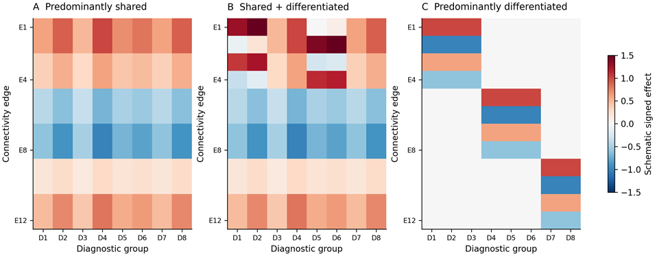
Figure 1. Schematic structural candidates in an age-overlapping population. Rows are connectivity features and columns diagnostic contrasts. A: one common-direction pattern with varying amplitudes. B: a common pattern plus differentiated components. C: several family-specific patterns. Colors depict signed effects, not observations. The diagrams do not establish reproducibility: “no structure above the floor” and “unresolved” are additional possible outcomes. Broad transfer must be tested independently rather than inferred from the visual average.

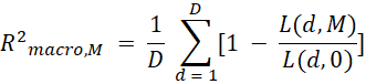
Define one primary score. For each disorder, average squared prediction error across its prespecified edges and eligible held-out sites, then divide by that disorder's zero-prediction loss. Average these normalized scores equally across disorders. This macro-averaged predictive R² prevents sample counts from determining the diagnostic weights. Do not compute an average of small, unstable fold-specific ratios: aggregate each disorder's out-of-fold losses before forming its ratio. Pooled-participant, precision-weighted, and ratio-of-macro-loss scores are sensitivity analyses with different targets.

R2macro,M = 1D d = 1D[1 - L(d,M)L(d,0)]

A noise ceiling is part of the result. Held-out effect maps contain sampling error and site-specific deviations, so even a perfect predictor of the reproducible population map cannot explain all observed variation. Estimate the reproducible signal energy from independent site partitions or cross-site products, with uncertainty, and normalize using the same per-disorder denominators and equal diagnostic weights as the primary score. Report each disorder's ceiling and the macro ceiling beside prediction scores. Within-site split halves measure sampling repeatability but retain shared site effects; they cannot by themselves establish an across-site ceiling. Resampling sites estimates uncertainty rather than proving that the ceiling has been identified.

The distinction changes interpretation. A low raw R² can capture a substantial fraction of a low ceiling; a larger R² can be inadequate when much more stable signal is available. Conversely, a small positive score with an imprecise or negligible reproducible signal estimate does not warrant a shared-architecture claim. Require both a prespecified minimum signal magnitude on the effect scale and a minimum fraction of the estimated ceiling. Test these jointly with uncertainty instead of dividing by an unstable ceiling estimate. Retain negative ceiling estimates in reports as evidence of estimation uncertainty; do not clip them to manufacture interpretable ratios.

Define outcomes before naming architectures. If neither candidate meets the evidence floor with adequate precision, a sufficiently informative upper-bound test can support “no reproducible structure above the specified resolution.” Otherwise the result is unresolved. This outcome is threshold-qualified: it does not establish that every connectivity association is exactly zero. Only after a model clears the floor should the comparison distinguish predominantly shared, shared plus differentiated, and predominantly differentiated structure.

The floor is an inferential commitment, not a universal numerical constant. Its magnitude should reflect the effects the study seeks to characterize and its fraction of recoverable signal. Noise ceilings, floors, and margins should be examined in design-calibration simulations before decisive data analysis. Supplementary Methods S2 gives explicit illustrative values for the computational experiment; those values are not proposed as standards for psychiatric imaging.

5. Compare structure without making sharing inevitable

The primary comparison asks whether differentiated components improve prediction meaningfully beyond one common-direction pattern. A rank-one model permits different diagnostic amplitudes along one edge pattern. The higher-rank model permits additional patterns. Rank, regularization, and any data-dependent preprocessing are chosen in inner site folds; outer test outcomes remain unavailable until models are frozen. Figure 2 shows the validation boundaries.

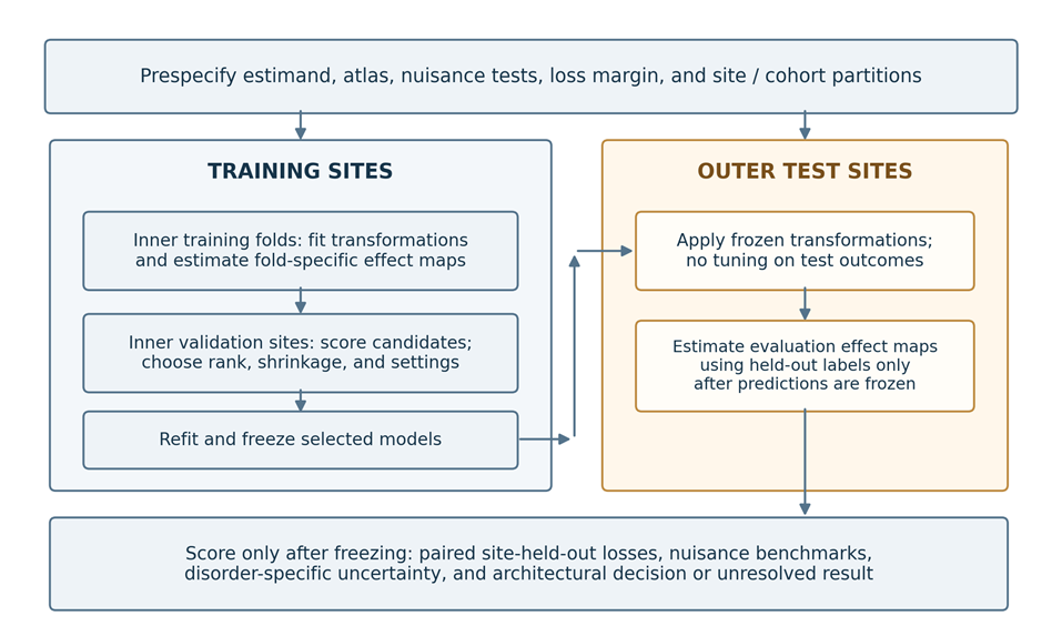
Figure 2. Site-based validation boundaries. Restrict or standardize to the target age distribution before defining the contrasts. Refit all learned transformations inside inner training folds; inner validation sites select settings. Refit on all outer training sites and freeze before scoring test effects. Test labels may construct evaluation contrasts but cannot update fitting. Keep overlapping participants and controls within their proper dependence structure. Noise ceilings and signed-transfer bounds are evaluation quantities, not permission to retune models.

Test sufficiency as non-inferiority. Let the gain be higher-rank minus rank-one predictive R², and define the tolerable gain as a prespecified fraction of the macro noise ceiling. Rank one is sufficient when it clears the evidence floor and the upper one-sided confidence bound for gain minus margin is below zero. A lower bound below minus the margin is harmless: it means rank one may perform better. A material higher-rank gain requires the corresponding lower bound to exceed zero. Propagate ceiling uncertainty jointly with gain uncertainty rather than replacing the ceiling with a fixed point estimate.

Δ = R2macro,H - R2macro,1,    δ = κ Cmacro,    U0.95(Δ - δ) < 0

Test broad loading in independent data. Nonnegative amplitudes are a fitting constraint, not evidence that every disorder shares the pattern. Learn a direction in training sites and evaluate unconstrained signed projections in held-out sites. Require simultaneous lower bounds to exceed a minimum amplitude on a clearly normalized effect scale, rather than checking whether fitted coefficients are positive. A diagnostic group with an imprecise projection cannot be counted as evidence of broad sharing. A precise upper bound below that amplitude can refute the claim that the selected direction applies to every targeted group.

Transfer across diagnostic families is a stronger complementary test. Learn the putatively shared direction without a prespecified family, then test its signed projection in that family at unseen sites. A collection of separate family-specific patterns can otherwise produce a positive grand-average direction. Families must come from independent clinical or genetic theory, not clusters discovered in the same connectivity data. If classifications change under defensible family definitions, the shared interpretation is correspondingly conditional. A failed transfer test concerns that learned direction; it does not exclude every possible common neural component.

Interpret the combination of tests. Predominantly shared structure requires a rank-one model above the floor, non-inferiority to higher rank, and evidence of broad transfer. Shared plus differentiated structure requires a meaningful higher-rank gain and a reproducible broadly transferring common term. Predominantly differentiated structure requires a meaningful higher-rank gain and sufficiently precise evidence against the specified broad-transfer claim. When transfer is merely imprecise, report an unresolved distinction between shared-plus-differentiated and differentiated structure. Failure to reject sharing is not evidence for sharing.

For a more detailed decomposition, remove the frozen common term and evaluate its conditional held-out contribution without allowing residual components to rotate into its place. Also examine a refitted alternative. These analyses characterize a specified statistical representation; rotational freedom means a factorization cannot establish unique biological mechanisms. Network localization remains a separate hypothesis, assessed through capacity-matched feature sets rather than inferred automatically from the number of components.

Estimation must preserve the dependencies in the data. Reused controls induce correlated diagnostic contrasts. Repeated scans and participants occurring in multiple source datasets also create dependence. Keep these observations within partitions and represent their sampling covariance. Comparisons based on within-site contrasts are preferable to pooled comparisons when diagnosis and scanner are entangled. If a contrast is absent from a training partition, it cannot be evaluated as though its disorder amplitude had been learned. Restrict the target set or mark the corresponding test unsupported.

6. What an eight-disorder simulation can distinguish

We implemented an illustrative Gaussian simulation with eight diagnostic groups, 12 sites, and 64 correlated connectivity features. Diagnostic coverage ranged from three to 12 sites. The rare group contributed 25 cases and 50 controls at each of three sites; other contrasts had 100–300 cases and 100–250 controls, except that four sites reused one local control group across diagnostic contrasts. Site-shared and contrast-specific random effects were added. Features had unit marginal participant variance and within-block correlation of 0.25. All effects referred to one common age window; the experiment does not simulate a developmental trajectory.

Gaussian group-mean draws exactly reproduce the contrast distribution of the specified Gaussian participant model without storing individual records. Generalized least squares used the known generating contrast covariance, followed by low-rank compression and shrinkage. Three outer folds held out four sites each, with one rare-disorder site per fold. Inner validation used the other two site blocks. Candidate ranks were one, two, three, four, and eight; shrinkage multipliers were 0.5, 0.8, and 1.0. Higher-rank selection excluded rank one so that its additional capacity could be compared directly with the constrained candidate.

Six generating scenarios represented no stable diagnostic effect, shared structure, common-plus-differentiated structure, four differentiated diagnostic families, a weak shared effect, and shared nuisance without a stable diagnostic effect. The nuisance scenario was also evaluated after oracle removal of its known template and measured amplitude. Each scenario used 200 independent repetitions. The seed, design, code, replicate-level scores, and complete decision definitions are supplied with the supplement. Choices were fixed for the reported run after implementation checks; this was not a preregistered study.

The illustrative evidence floor required mean reproducible signal energy above 0.0025, corresponding to a root-mean-square standardized effect of 0.05, and prediction above 20% of the macro ceiling. The non-inferiority margin was 10% of that ceiling. Broad transfer required lower signed-projection bounds above 0.02 with the direction normalized to unit root-mean-square edge loading. These choices demonstrate a decision procedure, not clinically established thresholds. Table 2 replaces the earlier stipulated example with calculated results.

Table 2. Calculated outcomes from the eight-disorder simulation

Scores are means across 200 independent repetitions per scenario. R² and ceilings use the same equal-diagnostic weighting. Negative ceilings are retained. Outcome counts follow the exploratory rule in Supplementary Methods S2; “no structure” means no reproducible structure above the specified floor. Higher-rank settings were selected inside inner folds. Oracle nuisance adjustment uses the known generating nuisance term. Monte Carlo standard error for a proportion is at most 3.54 percentage points at 200 repetitions; these counts are not validated inferential error rates.

Under the strong shared generator, rank one was sufficient in all repetitions, but only 180/200 met the separate broad-transfer requirement. Under the mixed generator, higher rank improved prediction in all repetitions; 138/200 met broad transfer and 62/200 remained unresolved. Differentiated families were identified in 196/200 repetitions. Thus good rank discrimination did not guarantee precise attribution of the common component. No architecture was selected in the null or weak-shared scenarios; the weak signal had an estimated macro ceiling near 0.031 and generally fell below the declared signal floor.

The nuisance-only condition was detectable and rank-one sufficient in every repetition, with mean rank-one R² of 0.569. Broad transfer passed in 21/200 repetitions, even though the diagnostic effect was zero by construction. After oracle nuisance removal, 199/200 repetitions supported no residual structure above the floor. This contrast shows why ceilings and reproducibility cannot by themselves identify psychiatric biology. The estimated ceilings were close to the generating oracle ceilings in the strong-signal scenarios, but individual low-signal estimates were unstable. Full outcome counts, Monte Carlo variability, and disorder-specific ceilings are reported in Supplementary Methods S3.

The experiment establishes limited discriminability, not validation of the entire framework. The Gaussian design, known covariance, fixed family definitions, and oracle nuisance removal favor interpretability. Confidence bounds resample held-out sites conditional on fitted models; they do not include refitting uncertainty, and their nominal coverage is not established. The repetition-to-repetition distribution includes rerunning model selection, but that does not repair the within-repetition interval limitation. Broad-transfer bounds likewise use an approximate small-site procedure. Classifications are therefore exploratory operating characteristics of this implementation, not validated error-controlled decisions.

For an initiative-specific power study, replace these favorable assumptions with estimated acquisition effects, realistic missingness, diagnosis-by-age interactions, alternative family structures, more heterogeneous edge covariance, and nuisance measurement error. Refit the full pipeline inside inferential resampling where feasible. Vary the signal floor and ceiling-scaled margin over a declared grid. Report false selection and unresolved rates rather than highlighting only settings where the intended architecture wins. The present experiment makes the consequences of these choices visible and supplies a reproducible starting point.

7. The main threats to interpretation

Site and diagnosis. Common preprocessing reduces analytical differences but cannot make scanners, protocols, or recruited populations identical. ComBat-based approaches can reduce site effects while preserving specified biological covariates [22]. Including diagnosis is ordinarily intended to preserve diagnosis-associated variation. With severe site-diagnosis confounding, however, disease and scanner effects may not be separately identifiable. No adjustment can recover information absent from the design. Traveling-participant research illustrates the distinction between measurement differences and sampling differences [23].

Report the site-by-diagnosis structure, prioritize within-site contrasts where possible, and compare conclusions across defensible site models and harmonization strategies. For prediction, fit transformations within training folds. A deployment pipeline cannot require the unknown test participant's diagnosis to harmonize that participant's scan. Applying a harmonizer to an unseen scanner also requires an explicit, validated strategy.

Shared nuisance as a competing architecture. A common pattern may arise because diagnostic groups share differences in motion, vigilance, medication exposure, or scan conditions relative to controls. This rival must be tested at the same level as the proposed common neural pattern. Add nuisance-only predictors of site-specific effect maps, using group differences in motion, usable duration, acquisition, and measured vigilance. Evaluate whether an architectural model improves held-out loss beyond this nuisance baseline. Report nuisance-adjusted scores with newly estimated residual ceilings; an unadjusted ceiling cannot be reused after changing the target.

Estimate motion-, vigilance-, and global-signal-associated edge maps in independent reference data, or exclusively within each training partition, using the same atlas and processing choices. Compare the common map with these benchmarks using topology-aware nulls and site resampling; assess incremental held-out prediction after nuisance modeling. Vigilance templates validated with EEG or eye tracking are preferable to proxies derived from the same fMRI features being tested. Nuisance signatures are diagnostic benchmarks rather than perfect negative controls: arousal and global signal contain genuine neural variation. Template similarity is a reason to investigate attribution, not proof that all shared effects are artifacts.

Repeat the comparison in within-site case-control contrasts and motion-matched subsets, with retained duration matched or modeled. Match on nuisance measurements without using the connectivity outcome, and report changed sample composition and precision. Permute diagnostic labels within eligible sites under an exchangeability scheme consistent with covariates and shared controls, rerunning the full selection procedure. These null analyses check spurious structure; they cannot remove unmeasured confounding. A shared interpretation is strongest when it transfers across sites, adds to nuisance prediction, and remains compatible with the matched-subset estimates.

Motion, physiology, and arousal. Participant-level denoising and quality control are essential; a group covariate for mean displacement is insufficient [24]. Report residual artifact, retained duration, and exclusions by group. Vigilance drifts during resting-state acquisition can change connectivity [25]. Record or recover eyes-open/closed instructions, scan timing, recent sleep, sedating medication, and any EEG, eye-tracking, respiratory, or cardiac measurements. Where available, examine awake-only segments and physiology-adjusted analyses. Without direct vigilance measurements, report the residual ambiguity rather than treating a proxy as complete control. Quality exclusions can also disproportionately remove younger or more impaired participants, altering the target population.

Global signal regression. Global signal contains multiple sources of variation, and its regression changes the quantities being estimated [26]. Prespecified analyses with and without regression can assess robustness, but disagreement requires explanation rather than a vote between pipelines. Global effects should not automatically be labeled artifact, nor should their removal automatically be treated as proof of neural specificity.

Medication, comorbidity, and illness course. Medication exposure is entangled with indication, severity, chronicity, and treatment response. Adjusted associations and unmedicated subgroup analyses remain observational. Comorbidity should likewise be addressed through defined questions: the total association of a diagnosis and its association conditional on co-occurring conditions are different estimands. Missing medication or symptom measures require explicit reporting; imputation cannot manufacture an entirely unmeasured construct.

Development and representativeness. The age-overlap restriction in Section 4 is part of the primary matrix definition, not an optional covariate adjustment. Report the site-by-disorder-by-age support and effective sample after restriction. In age-band extensions, use the same target age distribution for every diagnostic contrast within a band, and do not fill absent columns by extrapolation. Distinguish age differences between people from within-person change. Geographic breadth also does not guarantee representativeness; report coverage and test supported subgroups.

Analytical flexibility and parcellation. Fix the primary atlas, resolution, subcortical coverage, network assignments, and connectivity estimator. Include a small, prespecified set of alternative resolutions and atlas families. Independently defined atlases reduce circularity; data-adaptive parcellations must be learned within training folds. Compare architecture at each atlas's native resolution, then compare mapped network-level summaries rather than correlating incompatible edge vectors. A component confined to one parcellation has limited evidence of robustness. Define the targeted multiverse before inspecting the decisive results. Specify primary pipelines, justified alternatives, outcome families, and how robustness will be summarized. All feature selection, dimensionality reduction, tuning, and data-dependent preprocessing must respect validation boundaries [27]. A result that appears only in one favorable pipeline requires a narrower claim.

Within-disorder heterogeneity. Group means are valid estimands without assuming that every patient has the same abnormality. They nevertheless conceal the distribution of individual deviations: opposite changes can cancel, and a subgroup can drive a mean. As a complementary analysis, fit age- and covariate-conditional reference distributions to training reference participants and calculate individual deviation scores with predictive uncertainty. Rutherford and colleagues explicitly extended their normative resource to functional connectivity using Yeo-17 and Smith-10 network representations [28]. Compare deviation burden, spatial overlap, and symptom associations within and across diagnoses, rather than interpreting the mean map as a typical patient. Validate calibration in held-out reference participants and scanners; keep test cases out of reference fitting, and prespecify any separate calibration sample for a new site. An extreme deviation is neither a diagnosis nor evidence of pathology by itself, and a poorly representative reference can manufacture apparent abnormalities.

8. From scientific association to clinical value

A clinically useful imaging measure must answer a specific question, such as whether it improves prognosis, identifies people likely to benefit from a particular intervention, or monitors meaningful change. Case-control classification is often a weaker clinical target because diagnosis may already be available without scanning.

Begin with reproducibility and measurement quality. Establish that the relevant score or pattern can be estimated reliably enough for its intended use and that it generalizes beyond the development setting. Do not substitute the reliability of individual edges for that of the complete predictor, or assume that a reproducible artifact is valid.

Next establish incremental predictive value. Compare imaging with an appropriate clinical baseline, assess calibration as well as discrimination, and report uncertainty and subgroup performance. Required performance depends on the decision, prevalence, alternatives, errors, and costs.

Finally evaluate whether using the measure improves outcomes. A prognostic marker predicts outcome irrespective of treatment; a treatment-selection marker helps distinguish relative benefit between options. Treatment selection therefore requires evidence of differential treatment benefit, ideally from suitable randomized comparisons, followed by prospective evaluation of the decision strategy. Imaging-guided care should demonstrate benefits sufficient to justify burden, cost, and potential misclassification.

Dinga and colleagues' methodological replication of proposed depression biotypes illustrates why cluster discovery requires stability checks and independent validation [29]. It does not establish that every future subtype will fail. It establishes that attractive categories and apparent prediction are insufficient grounds for implementation.

9. Conclusion: identify the boundaries of generalization

Harmonized functional MRI will be most informative when its claims have explicit evidential boundaries. Establish the target population and recoverable signal before interpreting rank. Compare common and differentiated patterns on held-out sites, test sharing without using the constraints that fitted it, and distinguish diagnostic averages from individual deviations.

The simulation shows why these commitments matter: an analysis can be reproducible yet dominated by nuisance, a simple model can be sufficient only at the study's resolution, and sparse diagnostic coverage can leave transfer uncertain. An informative result may therefore be a shared pattern within one age window, differentiated structure within particular families, or a precise absence of recoverable structure above the chosen floor. Such boundaries give subsequent mechanistic and clinical studies a clearer question to test.

References

1. Sheehan, S. T. (2026, October 22). Global team launches largest-ever study of brain function across eight mental illnesses. Keck School of Medicine of USC. https://keck.usc.edu/news/global-team-launches-largest-ever-study-of-brain-function-across-eight-mental-illnesses/

2. National Institutes of Health. (2026). Global Initiative for Harmonized Functional MRI in Psychiatry. NIH RePORTER, project 11269134; award R01MH142539-01. https://reporter.nih.gov/project-details/11269134

3. Caspi, A., Houts, R. M., Belsky, D. W., et al. (2014). The p factor: One general psychopathology factor in the structure of psychiatric disorders? Clinical Psychological Science, 2(2), 119–137. https://doi.org/10.1177/2167702613497473

4. Kotov, R., Krueger, R. F., Watson, D., et al. (2017). The Hierarchical Taxonomy of Psychopathology (HiTOP): A dimensional alternative to traditional nosologies. Journal of Abnormal Psychology, 126(4), 454–477. https://doi.org/10.1037/abn0000258

5. Bonifay, W., Lane, S. P., & Reise, S. P. (2017). Three concerns with applying a bifactor model as a structure of psychopathology. Clinical Psychological Science, 5(1), 184–186. https://doi.org/10.1177/2167702616657069

6. Goodkind, M., Eickhoff, S. B., Oathes, D. J., et al. (2015). Identification of a common neurobiological substrate for mental illness. JAMA Psychiatry, 72(4), 305–315. https://doi.org/10.1001/jamapsychiatry.2014.2206

7. Menon, V. (2011). Large-scale brain networks and psychopathology: A unifying triple network model. Trends in Cognitive Sciences, 15(10), 483–506. https://doi.org/10.1016/j.tics.2011.08.003

8. Sha, Z., Wager, T. D., Mechelli, A., & He, Y. (2019). Common dysfunction of large-scale neurocognitive networks across psychiatric disorders. Biological Psychiatry, 85(5), 379–388. https://doi.org/10.1016/j.biopsych.2018.11.011

9. Xia, C. H., Ma, Z., Ciric, R., et al. (2018). Linked dimensions of psychopathology and connectivity in functional brain networks. Nature Communications, 9, 3003. https://doi.org/10.1038/s41467-018-05317-y

10. Kebets, V., Holmes, A. J., Orban, C., et al. (2019). Somatosensory-motor dysconnectivity spans multiple transdiagnostic dimensions of psychopathology. Biological Psychiatry, 86(10), 779–791. https://doi.org/10.1016/j.biopsych.2019.06.013

11. Cocuzza, C. V., Chopra, S., Segal, A., et al. (2026). Brain network dynamics reflect psychiatric illness status and transdiagnostic symptom profiles across health and disease. Nature Communications, 17, 6678. https://doi.org/10.1038/s41467-026-75585-6

12. Marek, S., Tervo-Clemmens, B., Calabro, F. J., et al. (2022). Reproducible brain-wide association studies require thousands of individuals. Nature, 603, 654–660. https://doi.org/10.1038/s41586-022-04492-9

13. Noble, S., Scheinost, D., & Constable, R. T. (2019). A decade of test-retest reliability of functional connectivity: A systematic review and meta-analysis. NeuroImage, 203, 116157. https://doi.org/10.1016/j.neuroimage.2019.116157

14. Writing Committee for the Attention-Deficit/Hyperactivity Disorder, Autism Spectrum Disorder, Bipolar Disorder, Major Depressive Disorder, Obsessive-Compulsive Disorder, and Schizophrenia ENIGMA Working Groups. (2021). Virtual histology of cortical thickness and shared neurobiology in 6 psychiatric disorders. JAMA Psychiatry, 78(1), 47–63. https://doi.org/10.1001/jamapsychiatry.2020.2694

15. Cheon, E.-J., Bearden, C. E., Sun, D., et al. (2022). Cross disorder comparisons of brain structure in schizophrenia, bipolar disorder, major depressive disorder, and 22q11.2 deletion syndrome: A review of ENIGMA findings. Psychiatry and Clinical Neurosciences, 76(5), 140–161. https://doi.org/10.1111/pcn.13337

16. Elliott, M. L., Romer, A., Knodt, A. R., & Hariri, A. R. (2018). A connectome-wide functional signature of transdiagnostic risk for mental illness. Biological Psychiatry, 84(6), 452–459. https://doi.org/10.1016/j.biopsych.2018.03.012

17. McTeague, L. M., Rosenberg, B. M., Lopez, J. W., et al. (2020). Identification of common neural circuit disruptions in emotional processing across psychiatric disorders. American Journal of Psychiatry, 177(5), 411–421. https://doi.org/10.1176/appi.ajp.2019.18111271

18. McTeague, L. M., Huemer, J., Carreon, D. M., Jiang, Y., Eickhoff, S. B., & Etkin, A. (2017). Identification of common neural circuit disruptions in cognitive control across psychiatric disorders. American Journal of Psychiatry, 174(7), 676–685. https://doi.org/10.1176/appi.ajp.2017.16040400

19. Yan, C.-G., Chen, X., Li, L., et al. (2019). Reduced default mode network functional connectivity in patients with recurrent major depressive disorder. Proceedings of the National Academy of Sciences, 116(18), 9078–9083. https://doi.org/10.1073/pnas.1900390116

20. Di Martino, A., Yan, C.-G., Li, Q., et al. (2014). The autism brain imaging data exchange: Towards a large-scale evaluation of the intrinsic brain architecture in autism. Molecular Psychiatry, 19(6), 659–667. https://doi.org/10.1038/mp.2013.78

21. ADHD-200 Consortium. (2012). The ADHD-200 Consortium: A model to advance the translational potential of neuroimaging in clinical neuroscience. Frontiers in Systems Neuroscience, 6, 62. https://doi.org/10.3389/fnsys.2012.00062

22. Yu, M., Linn, K. A., Cook, P. A., et al. (2018). Statistical harmonization corrects site effects in functional connectivity measurements from multi-site fMRI data. Human Brain Mapping, 39(11), 4213–4227. https://doi.org/10.1002/hbm.24241

23. Yamashita, A., Yahata, N., Itahashi, T., et al. (2019). Harmonization of resting-state functional MRI data across multiple imaging sites via the separation of site differences into sampling bias and measurement bias. PLOS Biology, 17(4), e3000042. https://doi.org/10.1371/journal.pbio.3000042

24. Ciric, R., Wolf, D. H., Power, J. D., et al. (2017). Benchmarking of participant-level confound regression strategies for the control of motion artifact in studies of functional connectivity. NeuroImage, 154, 174–187. https://doi.org/10.1016/j.neuroimage.2017.03.020

25. Tagliazucchi, E., & Laufs, H. (2014). Decoding wakefulness levels from typical fMRI resting-state data reveals reliable drifts between wakefulness and sleep. Neuron, 82(3), 695–708. https://doi.org/10.1016/j.neuron.2014.03.020

26. Murphy, K., & Fox, M. D. (2017). Towards a consensus regarding global signal regression for resting state functional connectivity MRI. NeuroImage, 154, 169–173. https://doi.org/10.1016/j.neuroimage.2016.11.052

27. Scheinost, D., Noble, S., Horien, C., et al. (2019). Ten simple rules for predictive modeling of individual differences in neuroimaging. NeuroImage, 193, 35–45. https://doi.org/10.1016/j.neuroimage.2019.02.057

28. Rutherford, S., Barkema, P., Tso, I. F., et al. (2023). Evidence for embracing normative modeling. eLife, 12, e85082. https://doi.org/10.7554/eLife.85082

29. Dinga, R., Schmaal, L., Penninx, B. W. J. H., et al. (2019). Evaluating the evidence for biotypes of depression: Methodological replication and extension of Drysdale et al. (2017). NeuroImage: Clinical, 22, 101796. https://doi.org/10.1016/j.nicl.2019.101796